
Run Bias Point for the nominal 4 V output. Open Divider tolerances.py in Project and run 4,096 reproducible trials with independent uniform ±5% resistor tolerances. The histogram shows the output distribution; the empirical CDF shows the fraction at or below each voltage. Console summaries compare sample percentiles with resistor worst-case bounds. Zip mode pairs the resistors in batches of 256.
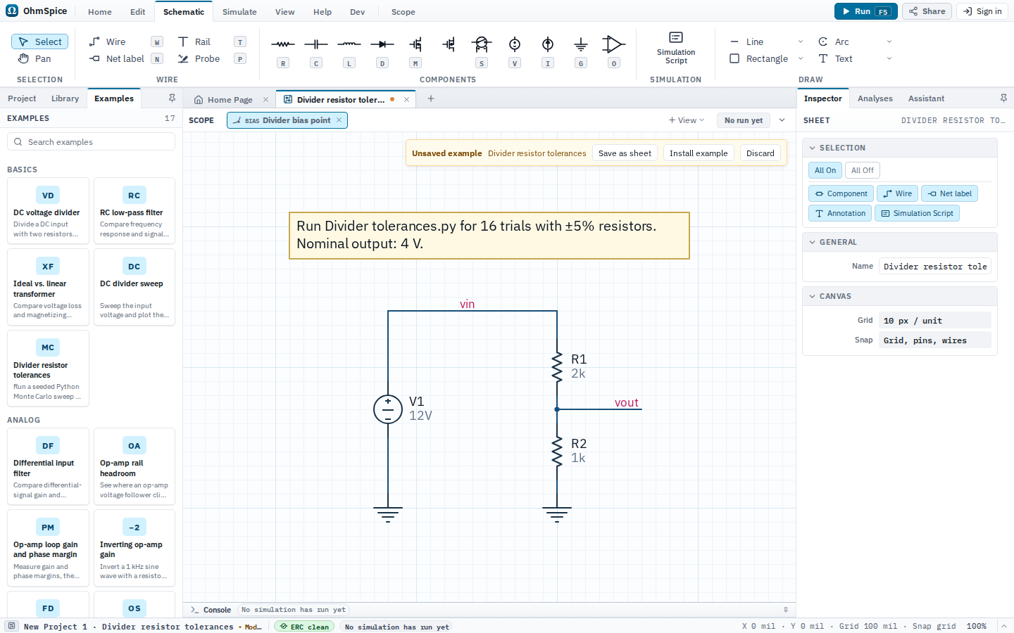
Open and run
- Open Examples from the Home ribbon.
- Choose Divider resistor tolerances.
- Open Simulate and choose Setup to review the analyses.
- Choose Run for one analysis or Run All for the complete configured set.
- Select a matching Scope view after the run. Use Save as sheet to keep the example or Discard to close it.
Sheets, analyses, and Scope
Divider resistor tolerances
Setup: Bias Point
| Analysis | Configuration |
|---|---|
| Bias Point | Default settings |
Scope views and expected results
Divider bias point
Analysis: Bias Point
Bias Point
V(vin)V(vout)
Readouts
- Output voltageLast
V(vout)
Python scripts
These scripts are included with the example. Review trusted project code before choosing Run.
Divider tolerances.py
Default sheet: Divider resistor tolerances
import numpy as np

sheet = get_sheet("Divider resistor tolerances")
samples = 4_096
batch_size = 256
rng = np.random.default_rng(42)
# Independent uniform tolerances are an assumption, not a measured population.
r1 = 2_000 * rng.uniform(0.95, 1.05, samples)
r2 = 1_000 * rng.uniform(0.95, 1.05, samples)
outputs = np.empty(samples)
# Zip pairs the resistors. Batches keep each sweep within its 256-run limit.
for start in range(0, samples, batch_size):
    stop = min(start + batch_size, samples)
    runs = sheet.sweep(mode="zip", R1=r1[start:stop], R2=r2[start:stop]).op(save="V(vout)")
    outputs[start:stop] = [run.v("vout").last for run in runs]
    print(f"Completed {stop:,} / {samples:,} trials")

nominal = 4.0
lower = 12 * 950 / (2_100 + 950)
upper = 12 * 1_050 / (1_900 + 1_050)
p01, p99 = np.quantile(outputs, [0.01, 0.99])
print(f"Mean {outputs.mean():.4f} V; sample standard deviation {outputs.std(ddof=1):.4f} V")
print(f"Sample 1st–99th percentiles: {p01:.4f}–{p99:.4f} V")
print(f"Resistor worst-case bounds: {lower:.4f}–{upper:.4f} V (fixed 12 V input)")

fig, axes = subplots(2, title="Divider tolerance distribution · 4,096 trials", sharex=True)
axes[0].hist(outputs, bins=48, range=(lower, upper), label="Independent ±5% resistors")
axes[0].set(xlabel="Output voltage (V)", ylabel="Trials per bin")
axes[1].ecdf(outputs, label="Empirical cumulative distribution")
axes[1].set(xlabel="Output voltage (V)", ylabel="Cumulative fraction")
for ax in axes:
    ax.axvline(nominal, label="Nominal 4 V")
fig.show()